An Information-Theoretic Definition for Open-Ended Learning

URL

Notes

Abstract

there is no coherent definition of open-endedness or theory about how an agent ought to explore an open-ended environment ()

bit-equivalent – which quantifies the information required to attain each level of expected reward ()

environment to be open-ended if an agent can attain linear growth in the bitequivalent ()

1 Introduction

environment as open-ended if the sequence of artifacts an agent produces is both novel and learnable, from the perspective of an observer ()

novelty means that there is greater uncertainty about future relative to current observations ()

learnable means that current observations inform predictions of future observations ()

novelty and learnability do not fully capture open-endedness ()

agent that continually generates novel and learnable policies does not necessarily acquire information that enables improved performance ()

environment open-ended if sustained reward improvement requires continual acquisition of useful information ()

bit-equivalent Bρ of expected reward ρ is the minimum amount of information about the environment required to attain expected reward ρ ()

agent achieves open-ended learning in such an environment if it realizes this linear rate (2)

example of an open-ended environment that is an infinite-dimensional linear-Gaussian bandit and establish that a variant of Thompson sampling achieves open-ended learning (2)

2 Problem Formulation

big-O notation to express asymptotic behavior of functions (2)

O ̃, when we choose to ignore logarithmic factors (2)

log to denote the natural logarithm (2)

random variables are defined with respect to a common probability space (Ω, F, P) (2)

bandit environment is defined by an action set A, an unknown parameter θ, a reward function r, and a noise distribution (2)

θ as a random variable (2)

time t ∈ N≥0 (2)

history Ht = (A0, R1, A1, R2, . . . , At−1, Rt) (2)

agent π (2)

action At ∼ π(· | Ht) (2)

reward (2)

Wt+1 is independent noise (2)

mean reward (2)

reward alone cannot distinguish between environments in which further improvement requires additional information and those in which it does not (2)

information-theoretic quantities in nats (2)

“bit-equivalent” where “bit” is used in the conventional sense to refer to information (2)

Definition 1 (Bit-equivalent)

bit-equivalent of expected reward level ρ ∈ R is (2)

I(θ; A) is the mutual information between θ and A in nats (2)

infimum is taken over all random variables A such that E [rθ (A)] ≥ ρ (2)

infimum: greatest lower bound.

Bρ is the amount information about θ required, on average, to select an action that delivers expected reward at least ρ (2)

performance of an agent π in terms of the average bit-equivalent (2)

Definition 2 (Average bit-equivalent)

average bit-equivalent of reward attained by an agent π up to time T is defined as (3)

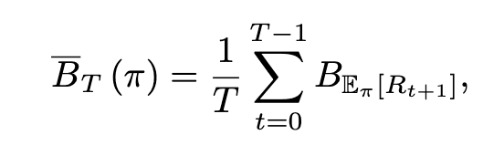
Eπ denotes the expectation over the randomness in θ, actions generated by the policy π, and the noise (3)

Definition 3 (Open-endedness)

environment is open-ended if there exists an agent π such that BT (π) = Ω(T ) (3)

3 Classical Bandit Environments Are Not Open-Ended

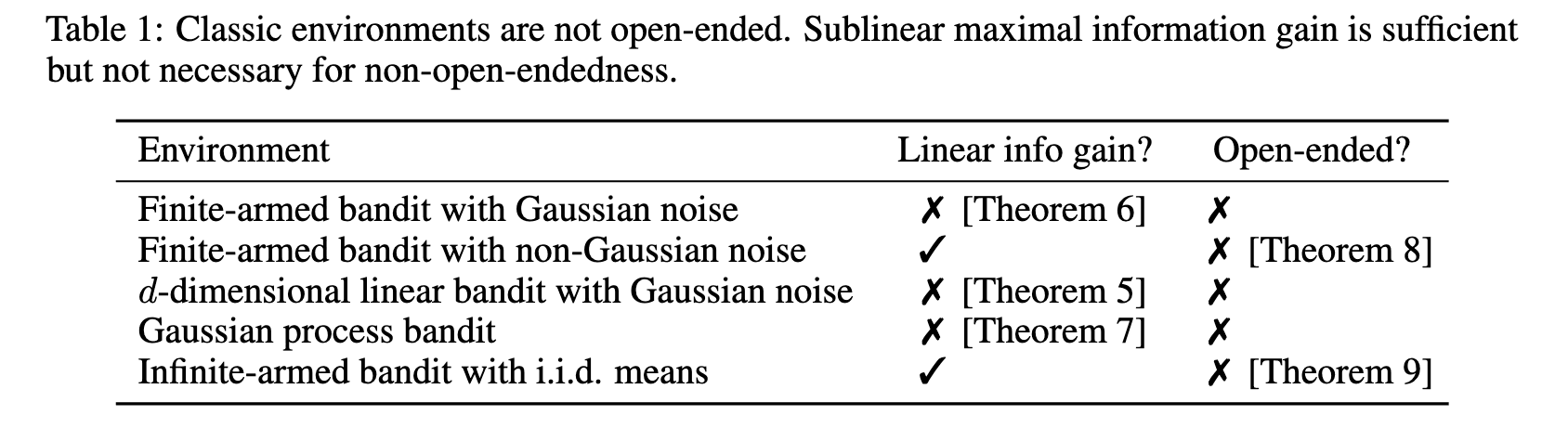
most classical bandit environments are not open-ended: either information about the environment cannot be acquired at a linear rate, or the information that can be acquired does not translate into sustained reward improvement (3)

information gain of an agent π up to time T (3)

upper bounds the average bit-equivalent (3)

all agents π and all T ≥ 1, BT (π) ≤ γT (π) (3)

The average bit-equivalent is upper bounded by information gain.

data processing inequality (3)

sublinear information gain for every agent implies non-open-endedness (3)

If we can prove that information gain is sublinear, we can say that environment is not open-ended.

sublinear information gain is sufficient but not necessary (3)

Sometimes, a non-open-ended environment can have infinite information gain also.

Therefore, it's not so straight forward to prove open-endedness using information gain idea.

So, we have average bit-equivalent idea.

3.1 Bandit environments with sublinear information gain

assume that the noise is additive Gaussian, i.e., rθ (At, Wt+1) = rθ (At) + Wt+1 and Wt+1 ∼ N (0, σ2) for some σ > 0 (4)

Finite-dimensional linear bandits

d-dimensional θ and A, and rθ (a) = θT a (4)

Theorem 5 (Information gain bound for linear bandits)

Finite-armed bandits

|A| < ∞ (4)

θ ∈ R|A| and rθ (a) = θa for all a ∈ A (4)

Theorem 6 (Information gain bound for finite-armed bandits)

Gaussian process bandits

infinite-dimensional analogue of finite-dimensional linear bandits (4)

"Infinite" dimensions is because of theta.

Theta is not a finite vector, it's a random function.

kernelized bandit optimization (4)

action set A ⊂ Rd is compact, the mean reward function rθ (a) = θ(a), and θ ∼ GP(0, k) is sampled from a Gaussian process with kernel k (4)

Gaussian Distribution: probability distribution over numbers. You get output as a number.

Multivariate Gaussian Distribution: Probability distribution over vectors. You get output as d-dimensional vector.

Gaussian Process: Probability distribution over functions. You get output as function.

Think of this function as an infinite dimensional vector, where each element in the vector can be seen as outputs of some single function with domain A (d-dimensional). When evaluated for every input from A we get an infinite dimensional vector like (f(a1),f(a2),...,f(ainf)).

GD: Mean, Variance

MGD: Mean Vector, Covariance Matrix

GP: Mean Function, Kernel

measure μ on A (4)

Mercer decomposition (4)

Eigendecomposition of a kernel.

eigenvalues λ1 ≥ λ2 ≥ · · · ≥ 0 (4)

functions {φm}m≥1 (4)

eigenfunctions.

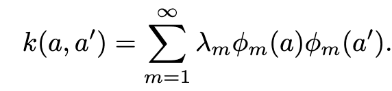
eigenvalues are summable (4)

spectral tail (4)

Theorem 7 (Information gain bound for Gaussian process bandits)

Matérn (5)

Even for an expressive kernel, the GP bandit remains non-open-ended.

squared exponential kernels (5)

Very smooth neighbor correlation.

3.2 Bandit environments where linear information gain does not imply open-endedness

acquire information at a linear rate, yet remain non-open-ended because this information does not support sustained growth in the bit-equivalent (5)

Finite-armed bandits with non-Gaussian noise

Unif([0, 1]) (5)

Uniform distribution on the interval [0,1]

finite action set itself imposes a stronger limitation: any action can be specified using at most log |A| nats of information (5)

Theorem 8.

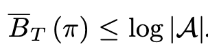
limitation of information gain as a proxy for open-endedness. The information gain γT (π) measures all information acquired about the environment, regardless of whether that information leads to high reward. By contrast, the bit-equivalent measures only the information required to select an action achieving a given reward level (5)

Infinite-armed bandits

Infinity is in the action space.

A is countably infinite (5)

Theorem 9 (Bit-equivalent bound for infinite-armed bandit).

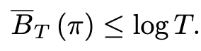
countably infinite actions alone does not imply open-endedness. For the commonly studied infinite-armed bandits with i.i.d. means, the average bit-equivalent achieved by any policy grows at most logarithmically (6)

4 An Open-Ended Environment

infinite-dimensional linear-Gaussian bandit (6)

Gaussian process bandit, but one that falls outside the standard kernel conditions (6)

insatiable linear bandit (6)

infinite-dimensional linear-Gaussian bandit.

A = a ∈ {0, 1}N : ∥a∥1 < ∞ . (6)

action is an infinite-dimensional binary vector with finite support (6)

θ ∈ RN (6)

θi ii∼d N (−1, 1) (6)

rθ (a) = ⟨θ, a⟩ (6)

additive Gaussian noise (6)

σ > 0 (6)

E[∥At∥0] < ∞ for all t (6)

In the coordinate basis, the kernel eigenvalues are not summable. This violates the spectral tail condition that rules out linear information gain (6)

The assumptions don't hold and del_D doesn't go to 0.

Theorem 10

insatiable linear bandit is open-ended (6)

insatiable logistic bandit (6)

This one doesn't have unbounded rewards, but still shows open-endedness.

rθ (At) = g(⟨θ, At⟩) (6)

g(x) = (1 + e−x)−1 (6)

4.1 Classical bandit algorithms fail to achieve open-ended learning

existing bandit algorithms are designed to operate in classical bandit environments (6)

two failure cases (6)

Algorithms that do not constrain the action set, such as Thompson sampling, attempt to explore too many coordinates (6)

TS agent.

Algorithms that truncate the action set to a fixed finite dimension limit the amount of information that can be extracted (6)

FT agent.

Thompson Sampling (TS)

πTS (6)

infinite-dimensional posterior over θ (6)

round t (6)

θ(t) ∼ P(θ ∈ · | Ht) (6)

action a (6)

maximizes a⊤θ(t) (6)

Theorem 11 (Thompson sampling failure)

all t ≥ 1 (7)

history Ht (7)

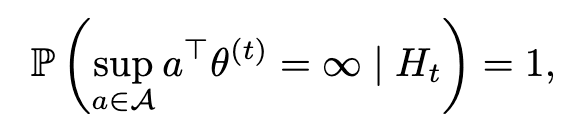
supremum is not attained by any action in A (7)

direct application of TS results in an ill-defined policy (7)

expected reward of the maximizer diverges to −∞ as the truncation approaches the full action set A (7)

Theorem 12 (Reward attained by Thompson sampling tends to negative infinity)

M ∈ N (7)

t ≥ 1 (7)

finite-dimensional truncation of A (7)

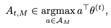
θ(t) ∼ P(θ ∈ · | Ht) (7)

history Ht (7)

Fixed Truncation (FT)

FT agent πM (7)

truncation window M ∈ N (7)

actions supported on the first M coordinates (7)

Theorem 13 (FT failure)

M ∈ N (7)

FT agent πM (7)

no fixed-M FT agent achieves open-ended learning (7)

4.2 Thompson sampling with a sequence of learning targets

agent should pursue a sequence of learning targets of increasing complexity (7)

first learns a simple target that supports modest reward, and then gradually moves to richer targets that support higher reward (7)

satisficing Thompson sampling (7)

modifies Thompson sampling by probability matching to an alternative learning target, such as a satisficing action, rather than to the optimal action (7)

Satisficing TS.

learning targets through a rate-distortion tradeoff (7)

not chosen to trade off a fixed information cost against a fixed approximation error, but rather to increase in complexity over time so that the agent can sustain linear growth in reward-relevant information (7)

Rate-distortion tradeoff modified to consider increase in information complexity over time.

learning target is a random variable χ (8)

represents partial information about the environment parameter θ (8)

optimal action (8)

a∗(χ) is the best action an agent could choose if it knew χ (8)

At time t, given history Ht, the agent samples χt ∼ P(χ ∈ · | Ht), and then selects an action At ∈ a∗(χt) (8)

Thompson sampling with learning target χ (8)

TS with learning target.

sequence of learning targets χ1, χ2, . . ., where later targets encode increasingly rich information about the environment (8)

time t, the agent chooses an index mt and applies Thompson sampling with respect to the target χmt (8)

At ∈ a∗(χmt t ) (8)

schedule mt is to balance two competing goals: the target χmt should be rich enough to support high reward, but simple enough that it can be learned effectively from data collected so far (8)

4.3 Truncated Thompson sampling achieves open-ended learning

insatiable linear bandit, the natural learning targets are finite-coordinate truncations (8)

χm = θ1:m (8)

Thompson sampling with target χm is therefore equivalent to running Thompson sampling on the truncated action set (8)

Truncated Thompson Sampling.

χm reveals the first m coordinates (8)

Truncated Thompson sampling (TTS) applies this idea with a truncation level that may grow over time (8)

round t (8)

history Ht (8)

truncation level mt = mt(Ht) (8)

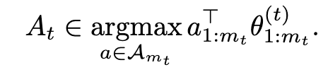
TTS avoids both the invalidity of full Thompson sampling and the bounded performance of any fixed truncation (8)

Because vannila TS agent gets -inf rewards, and FT agent rewards are bounded.

Theorem 14 (TTS success)

truncation schedule (mt)t≥0 (8)

TTS agent πTTS (8)

all T ≥ 1 (8)

TTS achieves open-ended learning (8)

average bit-equivalent rate achieved by TTS is optimal (8)

Theorem 15.

all T ≥ 1 (8)

all agents π (8)

algorithms for open-ended environments involves carefully thinking about the learning target (8)

GP-UCB-type agents (8)

Gaussian Process Upper Confidence Bound algorithm. 

One of the algos for Gaussian Process Bandit environment.

tuned confidence widths may also achieve open-ended learning (8)

need to prescribe sequences of learning targets or confidence set widths may render them fragile in practice (8)

TTS agent and GP-UCB-type agent.

5 Discussion

prior work, which largely focuses on empirical designs of open-ended agents and environments, as well as a small handful of recent papers attempting to formalize open-endedness (9)

5.1 Related work

Open-endedness in artificial life and AI

Formal definitions of open-endedness

Reinforcement learning and continual learning

Intrinsic motivation and curiosity-based methods encourage agents to explore by rewarding heuristics of uncertainty and novelty (9)

Hierarchical RL approaches the problem of open-ended learning via temporal structure discoveries (9)

Continual learning studies agents that learn over indefinite interaction and may face changing or expanding tasks (9)

Classical bandits and unbounded rewards

While unbounded rewards and infinite action sets may appear to provide natural sources of open-endedness, we show that neither is sufficient (9)

open-endedness requires that useful information about the environment can be continually acquired to sustain performance improvement (9)

5.2 Conclusion and limitations

First, our definition for openendedness applies only to the bandit setting (9)

Extending this definition to accommodate stateful and nonstationary environments is an important next step (9)

Second, as discussed at the end of Section 4.3, the TTS agent design requires as input a sequence of learning targets (9)

Designing agents without the need for deliberate hyperparameter choices is an exciting future direction (9)