Linear Transformers Are Secretly Fast Weight Programmers

URL

Notes

Abstract

“slow” neural net learns by gradient descent to program the “fast weights” of another net through sequences of elementary programming instructions which are additive outer products of self-invented activation patterns (today called keys and values) (1)

Slow Weights: Training Corpus Fast Weights: Test Time Input

replace the purely additive outer products by a delta rule-like programming instruction, such that the FWP can more easily learn to correct the current mapping from keys to values (1)

1. Introduction

core component of a Transformer is the self-attention mechanism (1)

self-attention computations scale quadratically with sequence length while the memory of the model grows linearly (1)

Vanilla Sa:

Time: O(n^2) Memory: O(n)

“linear Transformers” with constant size memory and time complexity linear in sequence length (1)

Linear Transformer:

Time: O(n) Memory: O(1)

complexity reduction is mainly due to a linearisation of the softmax (1)

memories of such FWPs contain key-value associations (1)

learn to reprogram them through sequences of differentiable elementary instructions (also called update rules) (1)

When the sequence length exceeds storage capacity, the model may end up in an overcapacity regime (1)

model should learn to dynamically interact with the memory contents and selectively decide which key-value associations to keep and which ones to delete (1)

purely additive instruction may be inappropriate (1)

introduce an improved programming instruction akin to the famous error-correcting delta-rule (1)

softmax linearisation techniques for Transformers are still underexplored (1)

l (1)

new method which is both simple and effective (2)

own synthetic retrieval dataset (2)

Dataset 1.

standard WMT14 English to German machine translation task (2)

Dataset 2.

Wikitext-103 (2)

Dataset 3.

2. Background on Fast Weight Programmers

general idea of fast weights is to make the weights also variable and input-dependent (2)

synaptic modulation (von der Malsburg, 1981), a method for variable binding in neural networks (see e.g. the recent survey by Greff et al. (2020)), or dynamic connections (2)

effective weights as a (multiplicative) superposition of conventional, context-independent slow weights, and fast changing, context-dependent fast weights (2)

slow net with slow weights continually changes or reprograms the fast weights of a fast net, making the fast weights effectively dependent on the spatio-temporal context of a given input stream (2)

Among the proposed elementary differentiable instructions that the slow net can use to program the fast weights, a particularly attractive one makes use of outer products (2)

Two vectors a and b:

Inner product: a dot b Output: Scalar

Outer product: a (x) bT Output: Matrix

FWP: Slow Weights Operation

FWP: Write Fast Weights by appending

FWP: Retrieval by matrix multiplication

⊗ denotes the outer product (2)

Forms a matrix.

σ is an activation function (2)

Wa and Wb are trainable slow weights (2)

fast weights W (i) are generated at each time step i (2)

Equivalent to short-term memory.

key-value associative memory model (2)

write operation is based on a summation (2)

W^(i)

retrieval is a matrix-vector multiplication (2)

y^(i)

use of outer products results in a model of associations similar to tensor product presentations (2)

Outer product organizes the associations in matrix form, meanwhile tensor product is simply more generalized (ex: collection of component multiplications in one vector).

associative memory can be found in numerous works (2)

Hebb’s informal rule (2)

Hopfield networks (2)

bi-directional associative nets (2)

concept of FWPs (2)

hypernetworks (2)

dynamic plasticity (2)

dynamic convolution (2)

lambda networks (2)

3. Relation to Transformers

3.1. Self-Attention Without Softmax Is a Fast Weight Programmer

self-attention layer in auto-regressive Transformers (2)

Autoregressive Transformer: 

Transformer generating sequence from left to right.

Autoregressive:

Regress the variable on the previous values of itself.

At timestep i: xi produces ki, qi, vi

Append the new key to previous keys

Append the new value to previous values

This is the KV cache

current query qi asks KiT qi (how relevant is current token to every token seen so far)

softmax of KiT qi given attention weights

Then, mix the corresponding values.

[A, a] denotes the concatenation of vector a to matrix A along the time dimension (3)

Wk, Wv, Wq are trainable weight matrices (3)

remove the softmax (3)

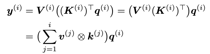
W (i) the corresponding weight matrix generated from key and value (3)

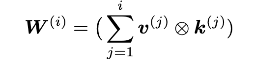
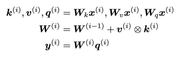
Self-attention as FWP.

3.2. Linearising Self-Attention

shown to improve computational efficiency of self-attention for long sequences (3)

softmax explicitly (3)

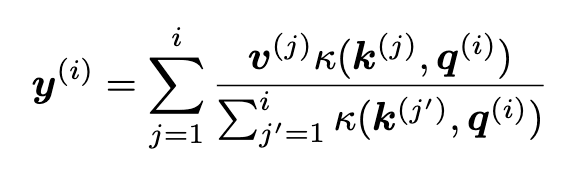
κ(k, q) = exp(k · q) ∈ R>0 is the softmax kernel (3)

k · q = k>q is the vector dot product (3)

replace the softmax kernel κ by another kernel: κ′(k, q) = φ(k)>φ(q) where φ is a function Rdkey → Rddot (3)

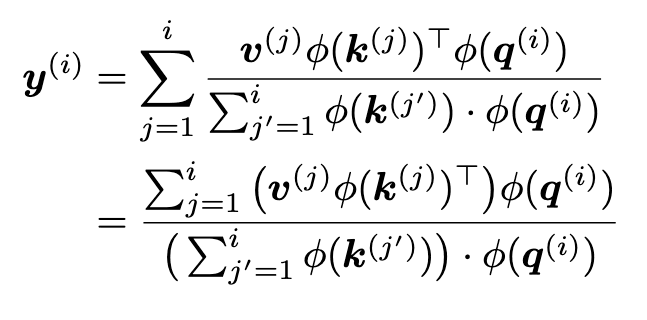
outer-product notation, the numerator is analogous to the case without softmax (3)

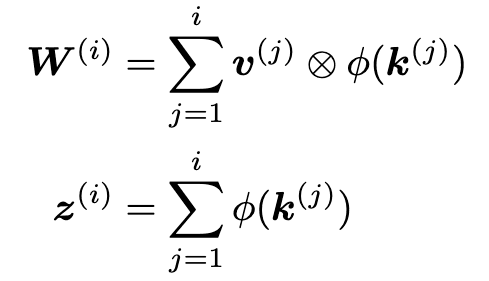
fast weight matrix W (i) (3)

additional vector z(i) (3)

forward computations of linear Transformers (3)

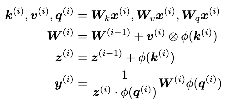
Linear Self-Attention as FWP with normalization.

4. Analysing and Improving Linear Transformers as Fast Weight Programmers

two insights (3)

their capacity limits as associative memories (3)

ineptness to edit previously stored associations (3)

4.1. Capacity Limitation

Intuition

Endlessly adding new associations to a memory of finite size, as in Eq. 17, inevitably will reach a limit (3)

W^i = W^(i-1) + v^(i) (x)  k^(i)

Here the fast weight matrix is endlessly added with the outer product.

linear attention, information is stored in a matrix and is retrieved using matrix multiplication (3)

y^(i) RHS is simply matrix multiplication and is the retrieval.

to prevent associations from interfering with each other upon retrieval, the respective keys need to be orthogonal (3)

keys embedded in a ddot space (3)

The phi kernel function output dimension is d_dot.

storing more than ddot associations will result in a retrieval error (3)

Association: a key-value pair.

when the length of the sequence is longer than ddot, the model might be in such an overcapacity (3)

Tensor Product Representation Theory

distributed representations as a means for storing symbolic structures (4)

Distributed representation: Concepts and entities are vectors and so information is spread across.

Symbolic structure: information represented as discrete entities and explicit relations between them.

tensor product representation (TPR) of a structured symbolic system consisting of a set of variables and values constructed from outer products of the so called role and filler vectors (4)

filler ((x)) role

Filler ~ Value Role ~ Key

Example:

"Peter loves MJ"

Roles are subject, verb, object. Fillers are Peter, loves, MJ.

Write: T = f_Peter r_subject^T + f_loves r_verb^T + f_MJ r_object^T

Read / Retrieval:

Subject: T dot r_subject

fast weight memories of Eq. 17 are the most basic form of such representations (second order tensors) (4)

Second order tensor is Matrix.

Smolensky (1990) discuss more formally the crosstalk and retrieval error intuitively (4)

The point on orthogonal associations and it is required to prevent interference.

classic TPRs of Smolensky (1990) are constructed with a priori knowledge of the symbolic structure (4)

TPR: Role (subject, verb, object) is from priori. 

FWP: Key itself isn't a priori.

4.2. Improving the FWP’s Programming Instruction

Once in overcapacity, an ideal memory model should dynamically interact with the memory contents and selectively determine which associations to remember or to forget (4)

contrast to the standard Transformer which stores immutable pairs (4)

from the perspective of dynamic interaction with the memory, the purely additive update rule of Eqs. 17 may be sub-optima (4)

basic instruction that essentially implements the famous error-correcting delta rule (Widrow & Hoff, 1960) in an end-to-end differentiable way (4)

Given a new input key-value pair (k(i), v(i)), the FWP first accesses the current state of the memory W (i−1) and retrieves the value v ̄(i) currently paired with the key k(i) (4)

Then the model stores a convex combination v(i) new of the retrieved value v ̄(i) and the input v(i) using an interpolation weight 0 ≤ β(i) ≤ 1 also generated by the model (4)

Retrieve v^(i) paired with k^(i)

Model generated the interpolation weight.

Model stores new value, which is a convex combination of retrieved value and input value.

beta (v - v_bar) + v_bar

first term is directly the error.

Wβ ∈ R1×d (4)

σ is the sigmoid function (4)

interpolation weight β(i) is the “write-strength” (4)

β(i) only depends on x(i) (4)

multilayer model, x(i) has the full context information (4)

W (0) = 0 (4)

Fast weight memory at timestep 0 is 0.

z(0) = 0 (4)

Accumulated normalization at timestep 0 is 0.

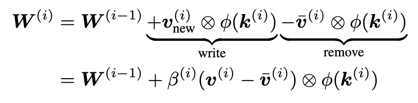
Delta Rule.

Final output.

dynamic learning rate β(i) (4)

advantage of this approach over the gated update rule (4)

Normalisation

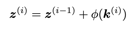
accumulator (4)

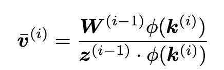
Value with normalization.

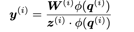
Output with normalization.

define v ̄(1) = 0. In this approach, the output y(i) is a weighted average of β(j)(v(j) − v ̄(j)) for 1 ≤ j ≤ i. We refer to this approach as attention normalisation (4)

drawbacks (4)

First, the accumulation of positive values in Eq. 26 always grows with the number of steps, and may result in instability (4)

Second, specifically for our update rule, this normalisation is not sufficient to balance the weights between write and remove operations (4)

better approach based on simple normalisation (5)

divide the effective key and query vectors φ(k(i)) and φ(q(i)) by the sum of its components (5)

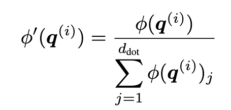
sum normalisation (5)

Divide the key and query vectors by sum of components.

Since this is a simple substitution of φ(k(i)) and φ(q(i)) in Eqs. 20-25, one might still ask whether additional attention normalisation is needed (5)

language modelling experiments (Sec. 6.3), we show that this is not the case (5)

5. Linear Attention Functions

softmax linearisation (Sec. 3.2) is the φ function which maps key and query vectors to the space where the dot product is executed: Rdkey → Rddot . (5)

5.1. Properties

φ should be positive (5)

dimensionality of its codomain ddot defines the model’s capacity (5)

transformation which projects the input dimension dkey to a larger dimension ddot, the φ function can potentially increase the upper bound (5)

5.2. Katharopoulos’ Linear Attention

simple element-wise ELU + 1 (5)

a simple element-wise function, this φ function preserves the dimension of the input key vector (dkey = ddot) (5)

5.3. FAVOR+

mathematically rigorous method to approximate the softmax with random features (5)

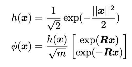
concatenation [a b ] of two vectors a and b (5)

R ∈ Rm×dkey is a matrix with m random features (5)

row vector r ∈ R1×dkey is drawn from N (0, Idkey ) (5)

dimension of the codomain ddot is 2m (5)

increases the theoretical capacity of the memory if 2m > dkey (5)

m is the only hyperparameter of FAVOR+ (5)

sampling process is the main drawback of FAVOR+ as it introduces variance into the model’s output (5)

5.4. Deterministic Parameter-Free Projection (DPFP)

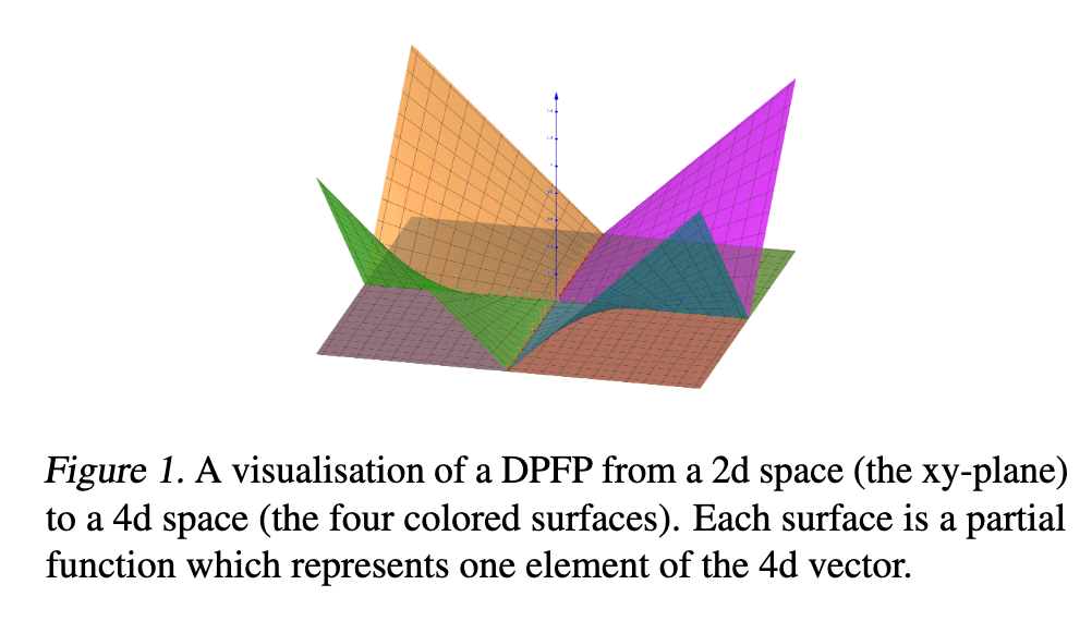
propose an alternative approach called deterministic parameter-free projection (DPFP) (5)

Consider 4 keys k(i), i ∈ {1, 2, 3, 4} in R2 (5)

φ : R2 → R4 ≥0 (5)

l-th element of φ(x) is generated by the partial function φl : R2 → R≥0 (5)

Partial function: takes the key in its d_key dimension and projects it onto a higher dimension d_dot

design φ such that it facilitates orthogonality in the projected space, i.e. φ(k(i)) · φ(k(j)) = 0 for i 6= j (5)

construct φ such that if φl(x) > 0 then φn(x) = 0 for all n 6= l (5)

enforced by limiting the domains of the partial functions to be non-overlapping (5)

For each phi_i ensure its domain doesn't overlap with others.

element-wise rectifier function r(a) = max(0, a) (6)

partial functions (6)

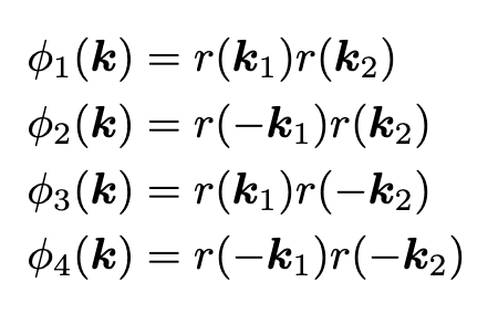
max(0,a) ensures only one of them is positive and makes rest 0.

phi = [ phi_1 phi_2 phi_3, phi_4]

phi: R2 to R4 phi_1: R2 to R1

for any k, find this projected components to be this.

each vector in the 2d plane will have a single non-zero component in the 4d space and equally splits the input space into four areas which will be orthogonal in the projected space (6)

input vector k ∈ Rdkey and i ∈ [1, 2dkey], the partial function (6)

i number of keys.

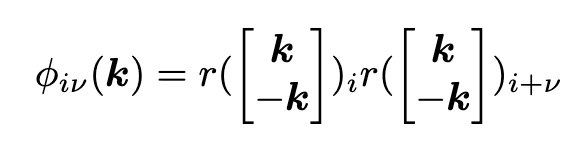
ν ∈ {1, 2, .., dkey2 − 1} is a capacity controlling hyperparameter (6)

Think of this as offset for doing element wise multiplication.

codomain dimensionality of φ(k) is thus ddot = 2dkeyν (6)

If we include more values for v, we are generating more sets of pairwise features.

6. Experimental Results

6.1. Synthetic Settings

our toy problem consists of retrieving the correct value from a sequence of randomly sampled keyvalue associations when queried with one of the used keys (6)

used key: key from the sampled keys value pairs.

K and V be the finite and fixed sets of keys and values (6)

S = |K| = |V| (6)

Total available keys and values.

input to the model is the sequence [(k, v)1, ..., (k, v)L] followed by q where every pair (k, v) ∈ K × V is sampled randomly, and q is randomly chosen to be one of the L keys (6)

Take L keys out of S.

v(i), i ∈ [1, .., S] is assigned a fixed one-hot vector v(i) ∈ RS (6)

The dimension of the one hot vector is the same as number of value vectors.

Hence, can have orthonormal basis.

embedding of the key symbols is the learned function e : K → Rdemb (6)

e is embedding function (learned).

k = WK [e(k); v] (6)

Write.

concatenate the value vector along with the embedding vector of key.

dim of e(k) is d_emb

dim of v is S (recall the orthonormal basis design requires that this should be S, the size of total key-value pairs)

WK ∈ Rdkey×(demb+S) (6)

d_key is the dim of key in this attention mechanism usage.

L write operations (6)

query vector q = WQe(q), WQ ∈ Rdkey×demb are used to retrieve vˆ ∈ RS from memory (6)

Retrieve.

loss is defined as l(vˆ, v∗) = ∑S j 1 2 (v∗ j − vˆj)2 (6)

v has S elements.

v∗ is the value vector assigned to q in the input sequence (6)

6.1.1. SETTING 1: TESTING CAPACITY

fix dkey to be 64 (6)

different φ functions produce different ddot (6)

L = S (6)

sample the keys and values without replacement (6)

all linear attention models (using the simple sum update rule of Sec. 3.2) fail at retrieving when S exceeds ddot. (6)

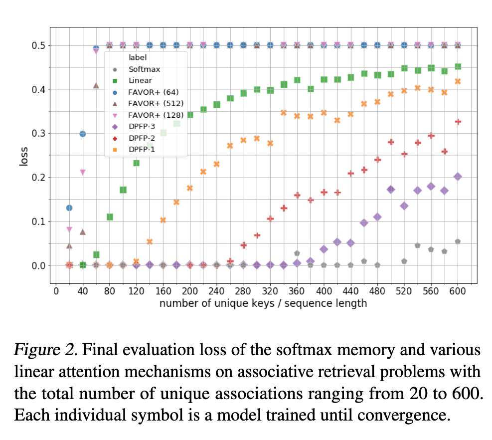
LinearAttention has a capacity of 64 due to the choice of dkey = ddot = 64. Experimentally, Linear-Attention begins to accumulate errors with 60 or more associations (7)

DPFP projections 1, 2 and 3 start to accumulate errors as they approach their respective limits at 128, 256, and 384 (7)

softmax attention is outperforming all φ functions, although it struggles to fully converge with more than 500 keys (7)

6.1.2. SETTING 2: COMPARING UPDATE RULES

keys and values will be sampled with replacement and sequence length L = 2S (7)

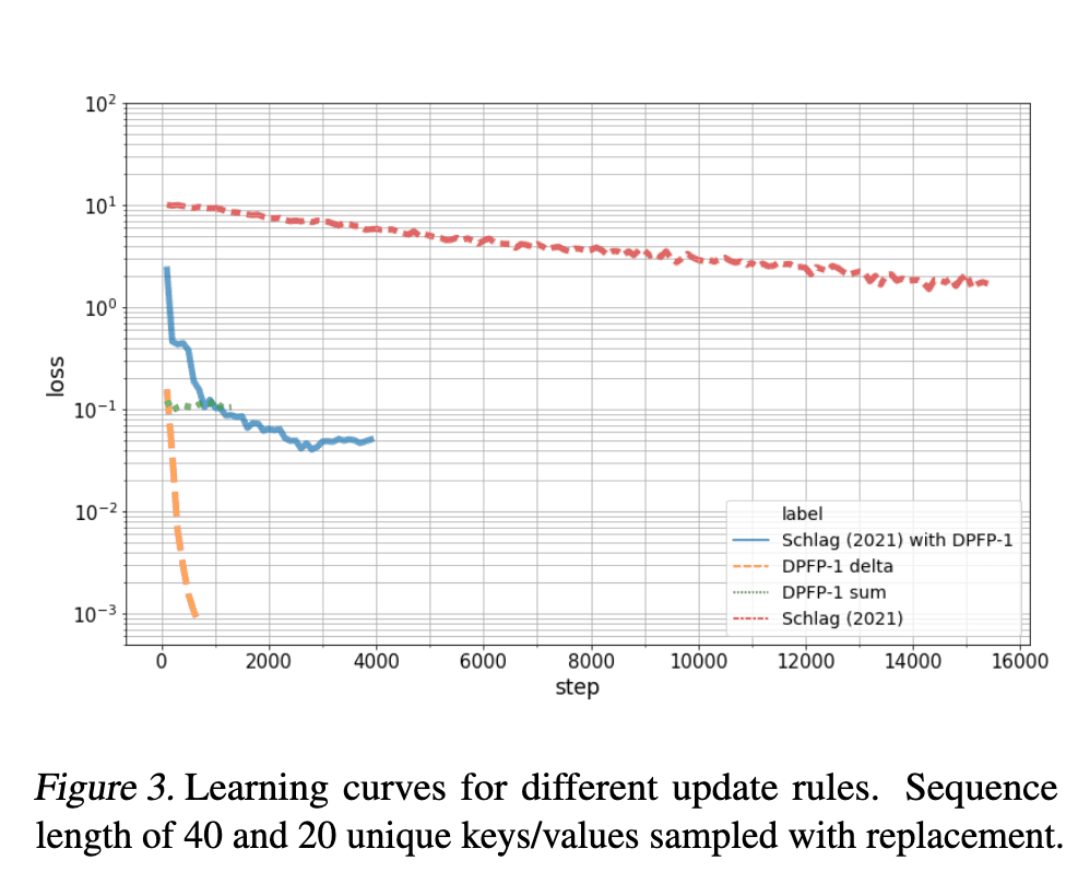
DPFP-1 as the φ (7)

sequence length is fixed at 40 with 20 unique keys and values (7)

fast weight memory programming instruction with normalisation (7)

three baselines (7)

sum update rule (7)

Schlag (2021) (7)

Schlag (2021) with DPFP (7)

tanh nonlinearity for its key representations (7)

new update rule outperforms all other variants (7)

6.2. Machine Translation Experiments

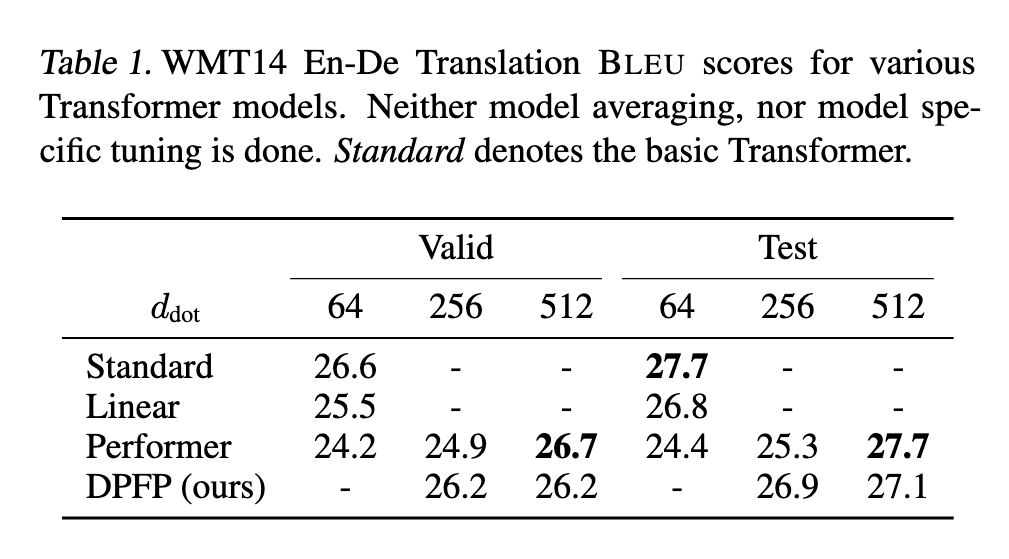
Linear Transformer (7)

Performer (7)

φ function DPFP (7)

vary the model hyper-parameters m in Performers (7)

ν in DPFP models (7)

BLEU score (7)

BLEU: Bilingual Evaluation Understudy

DPFP model outperforms the Linear Transformer as well as the Performer when ddot is relatively small (7)

6.3. Language Modelling Experiments

Experimental setups

WikiText-103 consists of long articles from Wikipedia (8)

training set contains about 28 K articles (8)

103 M running words (8)

contextual text blocks of about 3600 word (8)

validation and test sets (8)

218 K and 246 K running words (8)

split the training data into L-word long segments (8)

For evaluation, we use a batch size of one, and go through the text with a sliding window of size L (8)

only the last position for computing perplexity (8)

Perplexity: How surprised the language model is by actual next tokens.

Effectiveness of our new update rule

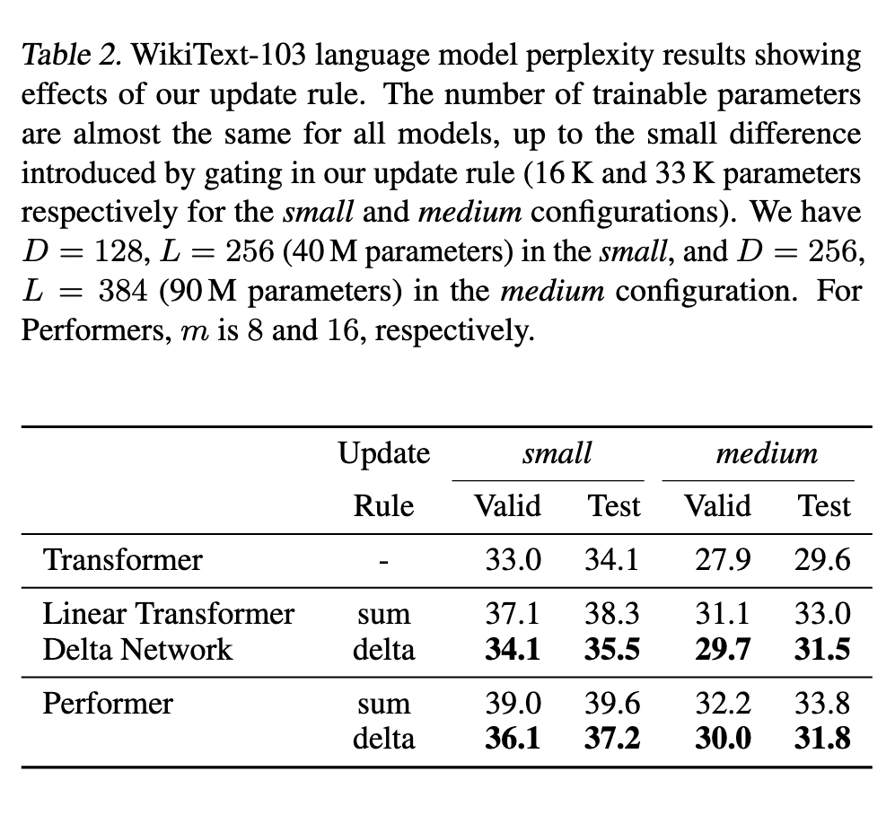
two configurations (8)

small configuration, we set the model dimension (same for key, value, and query) D to 128, and the training and evaluation context length L to 256 (8)

D = H ∗ ddot (8)

H is the number of heads (8)

H is set to 8 (8)

feed-forward layer dimension is 2048 (8)

medium configuration, we set D = 256 and L = 384 (8)

models can be trained using two V100 GPUs in less than four days (8)

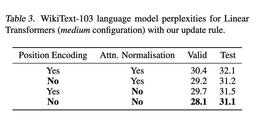
Linear Transformer with our delta update rule as a Delta Network (8)

ablation study to test the effect of the absolute positional encoding and an extra attention normalisation (8)

Ablation study: Remove or modify one of the components of a model to study performance changes.

better perplexities are obtained when no additional attention normalisation is applied (8)

Complexity, wall clock time, memory

All methods we propose are within the framework of “linear Transformers” (8)

constant in space (8)

The W^i matrix size is the same throughout the updates with outer product.

linear in time (8)

"The bird flew"

W^1: d^2 outer prod comp W^2: same W^3: same

Total is nd^2

So O(nd^2) = O(n)

63 K (9)

Wall Clock Time w Delta Rule.

66 K words/sec (9)

Wall Clock Time w/o Delta Rule.

14 (9)

Memory requirement w Delta Rule.

13 GB (9)

Memory requirement w/o Delta Rule.

extra resource requirement is thus marginal (9)

we use custom CUDA kernels for these linear Transformers, they are faster than the regular Transformers implemented in PyTorch which process 33K words/sec and require 17 GB memory (9)

speed of the DPFP and Performer models (for Table 5 in Appendix with a larger ddot) are 63 K and 57 K words/sec (9)

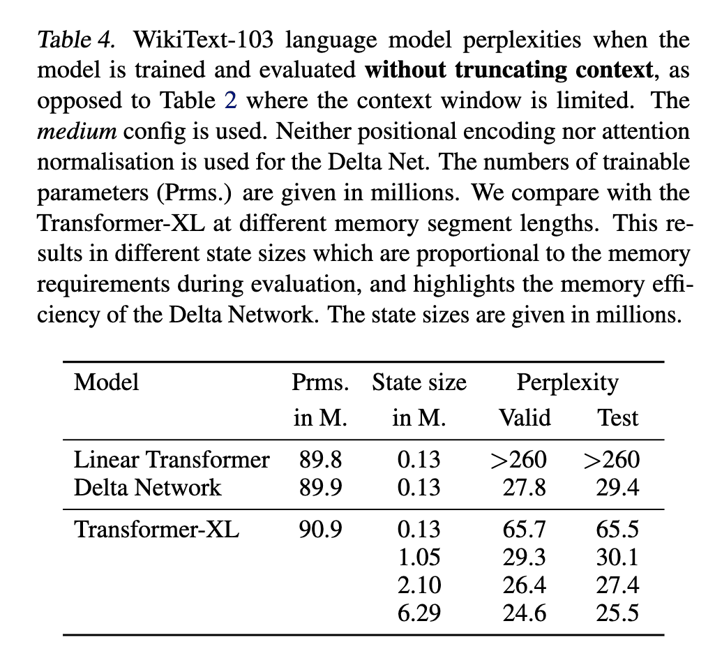
Without truncating context

Performance of the Delta Net does not yet match the performance of the Transformer XL when the latter is evaluated with a large state size (large attention window) (9)

7. Conclusion

FWP perspective allows for discussing associative memory capacity limitations of linear attention (9)

an alternative differentiable elementary programming instruction that the FWP can use to dynamically edit the memory, akin to the famous delta rule, but such that the FWP can learn to use the rule wisely through gradient descent (9)

Beta that decides the fast weights write strength comes from slow weights.

FWP perspective opens up new avenues for investigating even better programming instructions and designs for Transformers with finite memory (9)