CS168: The Modern Algorithmic Toolbox Lectures #11: Spectral Graph Theory, I

URL

Notes

1. represent the graph as a matrix ()

2. study the eigenvectors/eigenvalues of that matrix ()

we will consider undirected, and unweighted graphs (i.e. all edges have weight 1), that do not have any self-loops ()

Most of the definitions and techniques will extend to both directed graphs, as well as weighted graphs ()

1 Graphs as Matrices

Laplacian matrix associated to G is an n × n matrix LG = D − A ()

A derived matrix that aims to capture the local variation of node values (signals) on a graph

D is the degree matrix ()

Can be derived from matrix A

D(i, i) is the degree of the ith node (2)

A is the adjacency matrix (2)

Matrix A itself. Captures all about the connectivity of the graph.

A(i, j) = 1 if and only if (i, j) ∈ E (2)

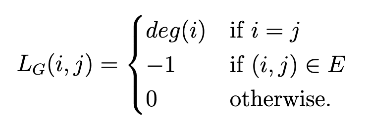
L_G is a matrix. Its elements are either deg(i) or -1 or 0.

consider what happens to a vector when we multiply it by L: if Lv = w (2)

deg(i)v(i): think of adding the v(i) for deg(i) times because deg(i) is the number of edges (i,j) going from node i

ith element of the product Lv is the sum of the differences between v(i) and the indices of v corresponding to the neighbors of i in the graph G (2)

quadratic form, vtLv (2)

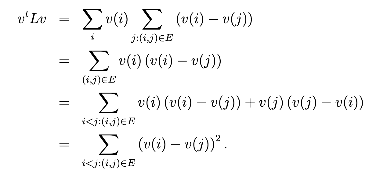
if one interprets the vector v as assigning a number to each vertex in the graph G, the quantity vtLv is exactly the sum of the squares of the differences between the values of neighboring nodes (2)

v is the value given (signal) on the nodes

if one were to place the vertices of the graph on the real numberline, with the ith node placed at location v(i), then vtLv is precisely the sum of the squares of the lengths of all the edges of the graph (2)

vTLv is a scalar called Dirichlet Energy

2 The Eigenvalues and Eigenvectors of the Laplacian

L is a real-valued symmetric matrix, all of its eigenvalues are real numbers, and its eigenvectors are orthogonal to eachother (2)

Because undirected graphs have symmetric information.

The eigenvalues of L contain information about the structure (or, more precisely, information about the extent to which the graph has structure) (3)

vTLv = Lambda_v * vTv

Collection of laplacian eigenvalues of a graph is called spectrum. 

Two graphs with the same set of spectrum are called co-spectral graphs.

Consider, the operation done on a graph that makes the original co-spectral with the output, that was a spectrum preserving operation and can tell things about the graph the spectrum could not reveal.

2.1 The zero eigenvalue

The laplacian always has at least one eigenvalue that is 0 (3)

Since every row and column of L sums to zero.

Operating L on any constant vector (every component is same) will result in a zero vector. Then that constant vector is the eigenvector with eigenvalue 0.

multiplicity of the zeroth eigenvalue reveals the number of connected components of the graph (3)

The number of zero eigenvalues of the Laplacian LG (i.e. the multiplicity of the 0 eigenvalue) equals the number of connected components of the graph G (3)

2.2 Intuition of lowest and highest eigenvalues/eigenvectors

vtLv = P (i,j)∈E,i<j(v(i) − v(j))2 is the sum of the squares of the distances between neighbors (3)

Sum of squares of edge lengths

eigenvectors corresponding to the lowest eigenvalues correspond to vectors for which neighbors have similar values (3)

vTLv is Lambda. Lambda is eigenvalue of eigenvector v

Eigenvectors with eigenvalue 0 are constant on each connected component (3)

say 6 nodes.

1-2-3  4-5-6

eigenvector (1,1,1,-1,-1,-1) with eigenvalue 0

1,1,1 is a constant vector -1,-1,-1 is a constant vector

smallest nonzero eigenvector will be the vector that minimizes this squared distance between neighbors, subject to being a unit vector that is orthogonal to all zero eigenvectors (3)

second smallest eigenvalue, because 0 is the smallest for every L

The maximum eigenvalue max||v||=1 vtLv will try to maximize the discrepancy between neighbors’ values of v (4)

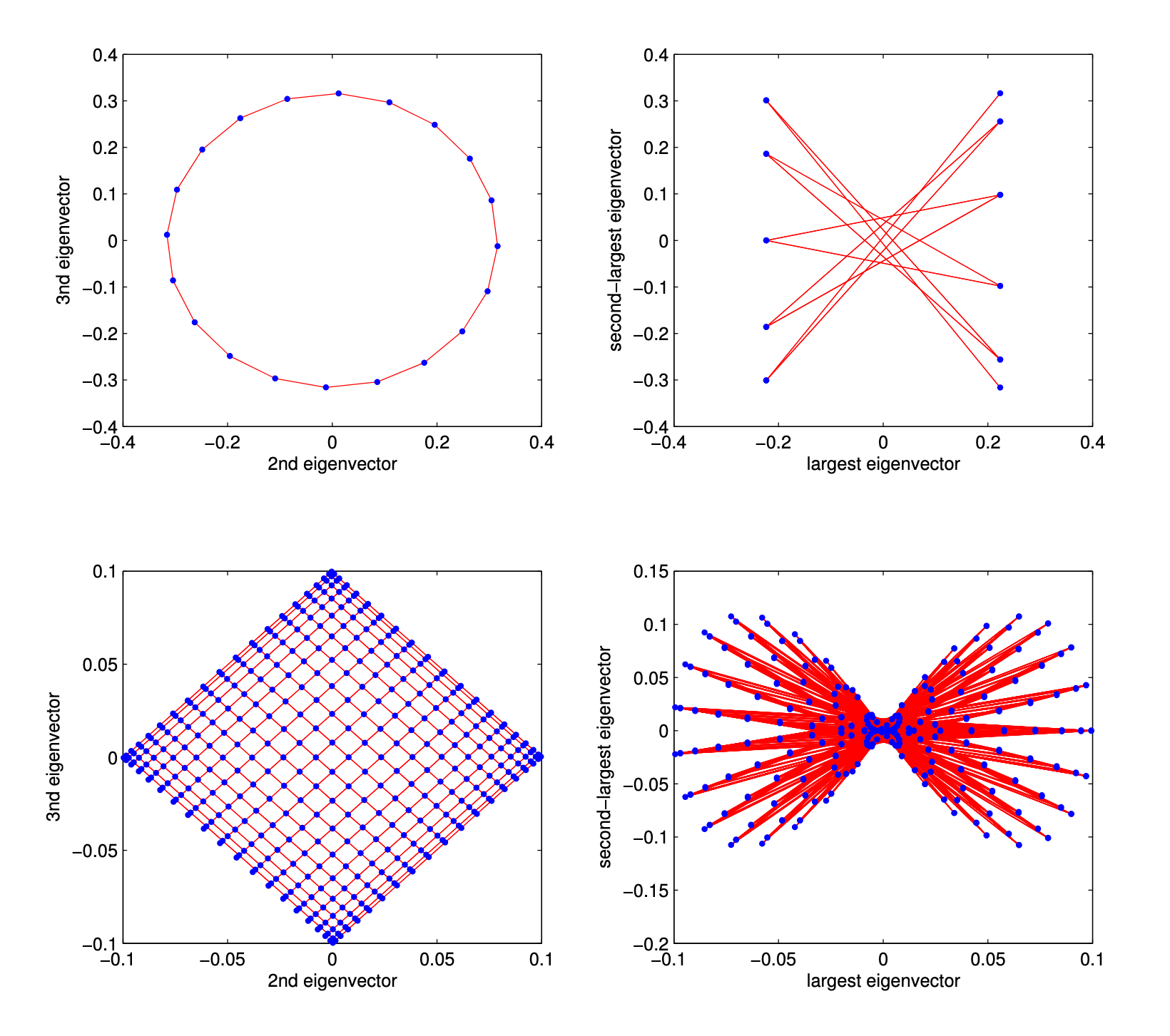
Spectral embeddings of the cycle on 20 nodes (top two figures), and the 20 × 20 grid (bottom two figures) (4)

The left two plots show the embeddings onto the eigenvectors corresponding to the second and third smallest eigenvalues; namely, the ith node is plotted at the point (v2(i), v3(i)) where vk is the eigenvector corresponding to the kth largest eigenvalue (4)

The right two plots show the embeddings onto the eigenvectors corresponding to the largest and second–largest eigenvalues (4)

3 Applications of Spectral Graph Theory

3.1 Visualizing a graph: Spectral Embeddings

the embedding onto the smallest two eigenvectors really does correspond to the “natural”/“intuitive” way to represent the graph in 2-dimensions (5)

Euclidean tools can be applied now.

3.2 Spectral Clustering/Partitioning

partition the graph into several large components so as to minimize the number of edges that cross between the components (5)

metrics for the quality of a given cluster or partition of a graph, and give some quantitative bounds on these metrics in terms of the second eigenvalue of the graph Laplacian (5)

eigenvectors corresponding to small eigenvalues are, in some sense, trying to find good partitions of the graph (5)

3.3 Graph Coloring

If two radio stations have overlapping regions of broadcast, then they cannot be assigned the same bandwidth (otherwise there will be interference for some listeners). On the other hand, if two stations are very far apart, they can broadcast on the same bandwidth without worrying about interference from each other (6)

problem of k-coloring a graph (6)

nodes of the graph will represent radio stations, and there will be an edge between two stations if their broadcast ranges overlap (6)

problem of finding a k-color, or even deciding whether a k-coloring of a graph exists, is NP-hard (6)

k-coloring heuristic as follows: (6)

1. plot the embedding of the graph onto the top 2 or 3 eigenvectors of the Laplacian (6)

2. locally partition the points in this space into k regions, e.g. using k-means, or a kd-tree (6)

3. assign all the points in each region the same color (6)