URL

Notes

CW complexes have proved over time to be the most natural class of spaces for algebraic topology (6)

algebraic topology separates naturally into the two broad channels of homology and homotopy (6)

tentatively titled ‘Spectral Sequences in Algebraic Topology’ and is referred to herein as [SSAT] (7)

vector bundles, characteristic classes, and K–theory, which will be largely independent of [SSAT] and also of much of the present book. This is referred to as [VBKT] (7)

reader should know about quotient spaces, or identification spaces (7)

∆ complexes, which are a mild generalization of the classical notion of a simplicial complex (7)

Homotopy and Homotopy Type

two spaces to be equivalent if they have ‘the same shape’ in a sense that is much broader than homeomorphism (10)

homeomorphism is a function to continuously deform one topological space to another, without tearing.

the "equivalent" is intended to be even broader. It's the homotopy.

thin letter is a subspace of the thick letter, and we can continuously shrink the thick letter to the thin one (10)

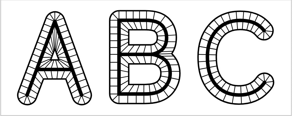
decompose a thick letter, call it X , into line segments connecting each point on the outer boundary of X to a unique point of the thin subletter X (10)

shrink X to X by sliding each point of X − X into X along the line segment (10)

<b>X</b> - X is the set theoretic difference

think of this shrinking process as taking place during a time interval 0 ≤ t ≤ 1 (10)

ft : X→X parametrized by t ∈ I = [0, 1] , where ft(x) is the point to which a given point x ∈ X has moved at time t (10)

deformation retraction of a space X onto a subspace A is a family of maps ft : X→X , t ∈ I , such that f0 = 11 (the identity map), f1(X) = A , and ft || A = 11 for all t (11)

Identity map here means output of the function is same as the input.

at t=0: the space X hasn't changed so f_0(x) = x

f_t|A: restrict the inputs to f_t from only space A then f_t(a) = a because space A is always fixed

ft should be continuous (11)

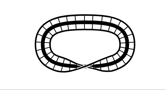
deformation retraction of a M ̈obius band onto its core circle (11)

Topology itself changed by deformation retraction.

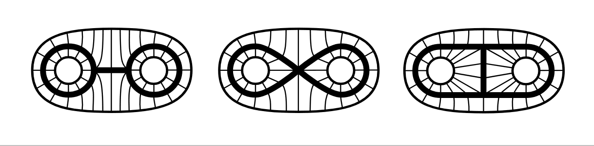
disk with two smaller open subdisks removed shrinks to three different subspaces (11)

Topology itself changed. Also, deformation retraction depends on the choice of space A, so not unique.

map f : X→Y , the mapping cylinder Mf is the quotient space of the disjoint union (X × I) ∐ Y obtained by identifying each (x, 1) ∈ X × I with f (x) ∈ Y (11)

mapping cylinder helps us convert the transformations (maps) into a thing (cylinder) that we can study.

I is unit interval [0,1] in topology

X x I because we want to thicken X into a cylinder first before we do quotient space (make some points equivalent), so we can also maintain a copy of X. here copy is (x,0)

Quotient space means we make points equivalent. In this case we make points (x,1) ~ f(x)

Quotient space is gluing.

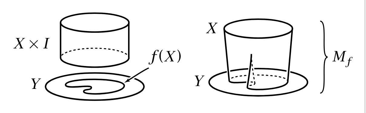
mapping cylinder Mf deformation retracts to the subspace Y by sliding each point (x, t) along the segment {x}× I ⊂ Mf to the endpoint f (x) ∈ Y (11)

thick X deformation retracts to the thin X , which in turn deformation retracts to the point of intersection of its two crossbars. The net result is a deformation retraction of X onto a point (11)

Thick X can be deformed to a point directly.

deformation retraction ft : X→X is a special case of the general notion of a homotopy, which is simply any family of maps ft : X→Y , t ∈ I , such that the associated map F : X × I→Y given by F (x, t) = ft(x) is continuous (12)

from space X to a different space Y.

X x I because I signifies t=[0,1] representation.

note: thick X to thin X to point is deformation retraction. Here its 3D to 2D to 1D. So,

• deformation retraction can collapse dimensions.
• deformation retraction must stay within its space of points.

Homotopy can describe maps that increase dimensions as well, and so entirely new space of points. like a 1D line segment to a 2D disk.

two maps f0, f1 : X→Y are homotopic if there exists a homotopy ft connecting them, and one writes f0 ≃ f1 (12)

that f_t is the homotopy (continuous path through space of maps from X to Y)

deformation retraction of X onto a subspace A is a homotopy from the identity map of X to a retraction of X onto A , a map r : X→X such that r (X) = A and r || A = 11 (12)

deformation retraction is a homotopy.

homotopy needs 2 endpoint functions f_0 and f_1. here:

f_0: identity map of X, f_0(x) = x f_1: retraction function of X onto A, f_1(X) = A and f_1(a) = a

we call f_1 as r (retraction function) such that:

r: X->X r(X) = A r | A = identity (note: we don't write it as r(A) = A, because its weaker. This would mean that the output belongs to the same space and nothing about the fixed / sameness of the output as the input point)

retraction as a map X→A restricting to the identity on the subspace A ⊂ X (12)

r: X->A r(X) = A r(a) = a for all a element of A

retraction is a map r : X→X with r 2 = r (12)

r^2 = r means r(r(x)) = r(x)

r is an idempotent function.

like the twin function for halfedge meshes.

Retractions are the topological analogs of projection operators (12)

projection operators try to project from some space to another.

say we apply some projection operator from R^3 to R^3. 

(x,y,z) -> (x,y,0)

Applying the projection operator again on the projection is just identity.

(x,y,0) -> (x,y,0)

space X always retracts onto any point x0 ∈ X via the constant map sending all of X to x0 , but a space that deformation retracts onto a point must be path-connected since a deformation retraction of X to x0 gives a path joining each x ∈ X to x0 (12)

retraction doesn't care about the line segments connecting the points in space X to A (that is path-connectedness).

but deformation retraction requires path-connectedness.

there are path-connected spaces that do not deformation retract onto a point (12)

homotopy ft : X→Y whose restriction to a subspace A ⊂ X is independent of t is called a homotopy relative to A , or more concisely, a homotopy rel A (12)

deformation retraction (f_t(a) = a and so obviously doesn't depend on t) is a special case of homotopy rel A (f_t(a) just doesn't depend on t).

the output points for inputs from subspace A of domain X, remain unchanged throughout the homotopy.

deformation retraction of X onto A is a homotopy rel A from the identity map of X to a retraction of X onto A (12)

more stronger statement on the kind of homotopy that happens with deformation retraction.

ft : X→X , then if r : X→A denotes the resulting retraction and i : A→X the inclusion, we have r i = 11 and ir ≃ 11 , the latter homotopy being given by ft (12)

we just view the space A points as space X points.

homotopy equivalence needs an inclusion function (and a retraction function of course).

r(i) is equal to identity (because no point has moved at all during this)

i(r) is homotopic to identity (because point has moved during this)

map f : X→Y is called a homotopy equivalence if there is a map g : Y →X such that f g ≃ 11 and gf ≃ 11 (12)

now generalize the deformation retraction case, relax the strict "equal to identity" for r(i) composition in deformation retraction, and make make both homotopic (the general homotopy case)

so now, fg and gf are homotopic to identity map and not necessarily equal.

the general version, functions f and g show homotopy equivalence.

special case: deformation retraction

• g can be the inclusion map. 
• f the retraction map.
• fg is then equal to identity.

spaces X and Y are said to be homotopy equivalent or to have the same homotopy type (12)

spaces X and Y are homotopy equivalent / show same homotopy type.

this is an equivalence relation, in contrast with the nonsymmetric notion of deformation retraction (12)

the three graphs are all homotopy equivalent (12)

say these are subspaces A, B, C of space X.

since this is deformation retraction case, there are 3 retraction maps and 3 inclusion maps.

Consider A and B,

A and B are homotopy equivalent because there can be f_AB and g_AB such that:

f_AB = r_B(i_A) such that A->B g_AB = r_A(i_B) such that B->A

now,

f_AB(g_AB) is homotopic to identity on B g_AB(f_AB) is homotopic to identity on A

therefore,

A and B are homotopy equivalent spaces.

two spaces X and Y are homotopy equivalent if and only if there exists a third space Z containing both X and Y as deformation retracts (12)

take Z to be the mapping cylinder Mf of any homotopy equivalence f : X→Y (12)

A space having the homotopy type of a point is called contractible (13)

identity map of the space be nullhomotopic, that is, homotopic to a constant map (13)

general identity map: f(x) = x nullhomotopic: f(x) = c

slightly weaker than saying the space deformation retracts to a point (13)

Because deformation retraction has strict constraints common to contractible:

f_0 = identity f_1 = constant map

and additionally,

f_t(a) = a.

• contractible: everything ends at x_0
• deformation retraction onto a point: everything ends at x_0 and x_0 never moves

example of a 2 dimensional subspace of R 3 , known as the house with two rooms (13)

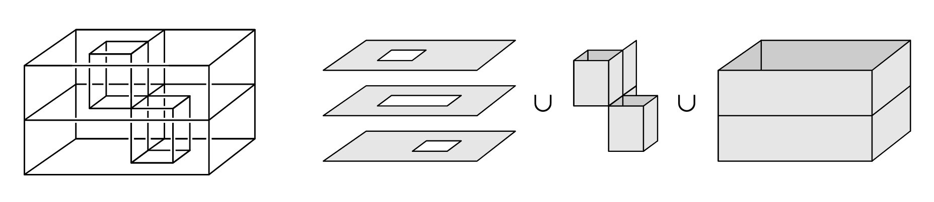
The resulting space X thus consists of three horizontal pieces homeomorphic to annuli plus all the vertical rectangles that form the walls of the two chambers (13)

consider a closed ε neighborhood N(X) of X . This clearly deformation retracts onto X if ε is sufficiently small (13)

Think of thickening the walls (this is deformation retraction which implies homotopy).

N(X) is homeomorphic to D 3 , the unit ball in R 3 (13)

Think of the fingers pushing and making space in a ball.

Lower finger makes the upper chamber space, upper finger makes the lower chamber space.

this is homeomorphism (this implies homotopy).

D 3 ≃ point (13)

Think of a ball deformation retract to a point (homotopy).

X is contractible (13)

House with 2 rooms is contractible.

X deformation retracts to a point (13)

House with 2 rooms is a deformation retraction onto a point.

Cell Complexes

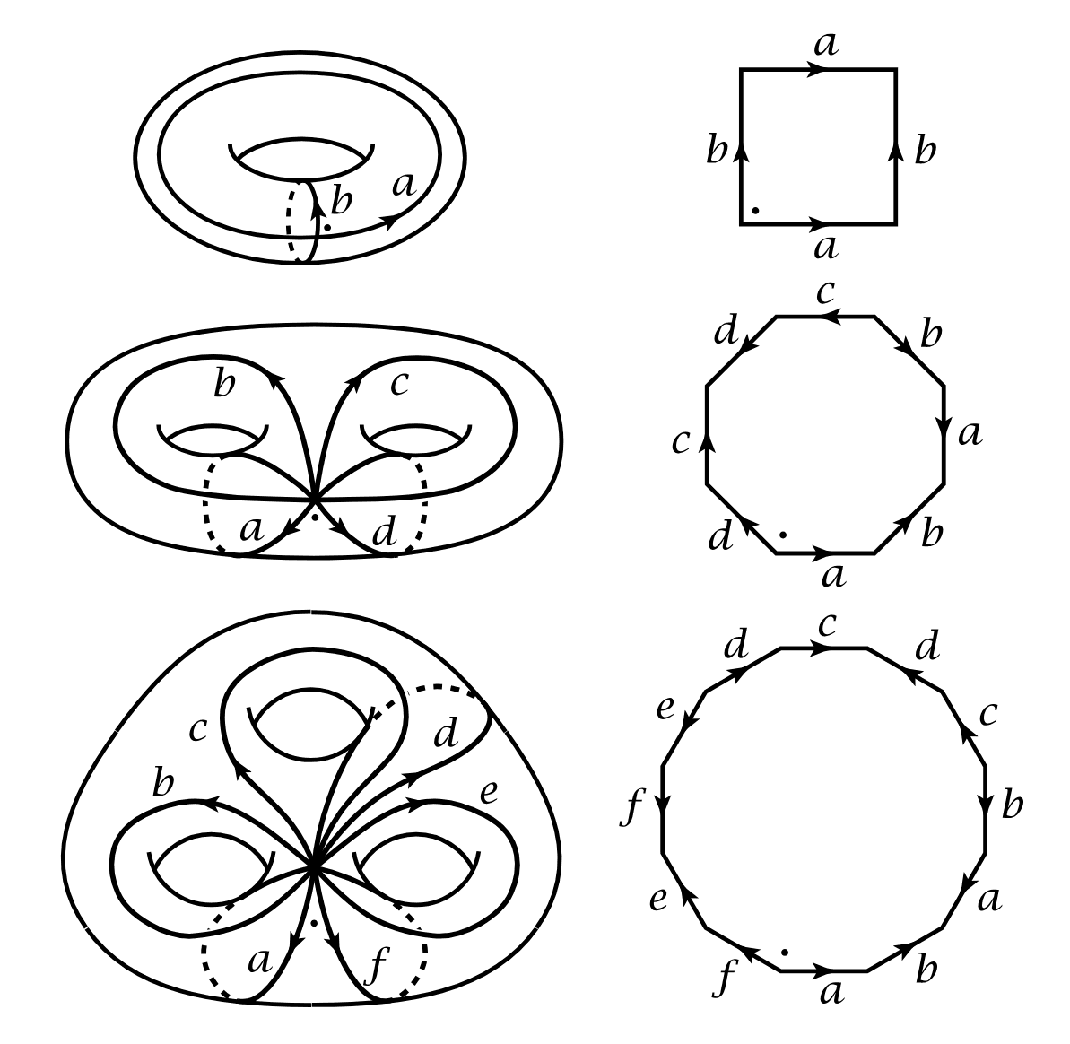
an orientable surface Mg of genus g can be constructed from a polygon with 4g sides (14)

genus is number of handles / holes

4g edges of the polygon become a union of 2g circles in the surface, all intersecting in a single point (14)

4g polygon on right. union of 2g circles on left.

The point is depicted in the figure.

interior of the polygon can be thought of as an open disk, or a 2 cell, attached to the union of the 2g circles (14)

2-cell: open disk

union of the circles as being obtained from their common point of intersection, by attaching 2g open arcs, or 1 cells (14)

1-cell: open arc

n cells eαn (14)

alpha-th n-cell.

alpha is the index given to the n-cell.

e^n = Interior(D^n)

maps φα : Sn−1→Xn−1 (14)

attaching map.

S^(n-1): boundary of new n-cell disk.

X^(n-1): space already built.

quotient space of the disjoint union X n−1 ∐ α Dαn (14)

gluing of these things in this union (which is disjoint as of now).

x ∼ φα(x) (14)

Rule for attaching.

attach x to attachingmap(x)

x ∈ ∂Dα (14)

point x is on the boundary of the disk.

n disks Dαn (14)

This has boundary + interior. boundary is required for attaching.

Xn = Xn−1∐ α eα (14)

X^n would simply be a union of n-cells.

one can continue indefinitely, setting X = ⋃ n Xn (14)

infinite cell complex.

A ∩ Xn (14)

Part of A that's in X^n.

open (or closed) in Xn for each n (14)

In each skeleton, A should be open.

space X constructed in this way is called a cell complex or CW complex (14)

Go skeleton by skeleton. You attach the n-cells to the entire X^(n-1) skeleton. And the entire boundary of the n-cell to be attached.

X = Xn for some n , then X is said to be finite-dimensional, and the smallest such n is the dimension of X , the maximum dimension of cells of X (15)

Dimension of a space is the smallest dimension among all possible CW decomposition.

Example: Dim(Standard Torus) = 2

1 dimensional cell complex X = X1 is what is called a graph (15)

Euler characteristic, which for a cell complex with finitely many cells is defined to be the number of even-dimensional cells minus the number of odd-dimensional cells (15)

even-dim cells - # odd-dim cells

Euler characteristic of a cell complex depends only on its homotopy type, so the fact that the house with two rooms has the homotopy type of a point implies that its Euler characteristic must be 1 (15)

sphere Sn has the structure of a cell complex with just two cells, e0 and en , the n cell being attached by the constant map Sn−1→e0 (15)

for a 2d sphere, we take all the boundary points of a closed disk 2-cell and glue them to one point, like a balloon.

Sn as the quotient space Dn/∂Dn (15)

/ means what's on RHS is equivalence.

Here, consider Set D^n, with every point in boundary set delD^n becoming equivalent to every other point in it. 

Now glue them all (quotient them) to a point (visualization).

Real projective n space RPn is defined to be the space of all lines through the origin in Rn+1 . Each such line is determined by a nonzero vector in Rn+1 , unique up to scalar multiplication (15)

Geometric Perspective.

Space of directions. Each point in the space is a line (gives direction). Like a vector without a magnitude.

RP^2: each point in this space is a line through origin in R^3.

RPn is topologized as the quotient space of Rn+1 − {0} under the equivalence relation v ∼ λv for scalars λ ≠ 0 (15)

Quotient of vectors.

All vectors on the same line becomes an equivalence class.

vectors of length 1 (15)

Push all those vectors in each equivalence class to unit distance from origin.

RPn is also the quotient space Sn/(v ∼ −v) (15)

Because we pushed, the only 2 representatives on the same line would then be diametrically opposite.

antipodal points (15)

if 3D, it's (x,y,z) & (-x,-y,-z)

RPn is the quotient space of a hemisphere Dn with antipodal points of ∂Dn identified (15)

Quotient of hemisphere.

hemisphere is homeomorphic to disk, and its boundary is a 2D disk.

So, 

RP^n is D^n / x~-x on delD^n

∂Dn with antipodal points identified is just RPn−1 (15)

By identified, we mean glued.

RPn is obtained from RPn−1 by attaching an n cell, with the quotient projection Sn−1→RPn−1 as the attaching map (15)

CW Complex.

S^1 is the regular boundary of a disk (ordinary colored rim).

RP^1 is the rim after antipodal points are attached (the mobius strip), this involves intersection.

RP^1 is just a circle. If given thickness it looks like mobius strip.

Keep increasing thickness. n-cell is disk interior which becomes the intersecting thing RP^2 (boy's surface).

RP∞ as the space of lines through the origin in R∞ = ⋃ n Rn (15)

Complex projective n space CPn is the space of complex lines through the origin in Cn+1 , that is, 1 dimensional vector subspaces of Cn+1 (15)

C^3 be (a+bi, c+di, e+fi)

Point in CP^2 would then be a line through (0,0,0) in C^3

quotient of the unit sphere S 2n+1 ⊂C n+1 with v ∼ λv for |λ| = 1 (16)

C^1 is 2 dimensional.

S^2n+1 because 2*(n+1) - 1 would be the dimension of the sphere for C^n+1.

CP n as a quotient space of the disk D 2n under the identifications v ∼ λv for v ∈ ∂D 2n (16)

D^2n because dimension of disk in C^n would be 2n.

graph of the function (16)

Set of (input, output) pairs.

CP n is obtained from CP n−1 by attaching a cell e 2n via the quotient map S 2n−1 → CP n−1 . So by induction on n we obtain a cell structure CP n =e 0 ∪e 2 ∪ ··· ∪ e 2n with cells only in even dimensions (16)

Each cell e n α in a cell complex X has a characteristic map Φ α :D n α → X which extends the attaching map φ α and is a homeomorphism from the interior of D n α onto e n α (16)

For an n-cell,

attaching map: boundary points characteristic map: boundary points + interior points

In case of RP^2 (boy's surface),

Where the points of the 2-disk ends up in the boys surface is the characteristic map of that 2-disk.

canonical cell structure on S n described in Example 0.3, a characteristic map for the n cell is the quotient map D n → S n collapsing ∂D n to a point (16)

The balloon visualization.

subcomplex of a cell complex X is a closed subspace A ⊂ X that is a union of cells of X (16)

closed: includes all of interior and boundary points.

A is a cell complex in its own right (16)

pair (X, A) consisting of a cell complex X and a subcomplex A will be called a CW pair (16)

natural inclusions S 0 ⊂S 1 ⊂ ··· ⊂ S n , but these subspheres are not subcomplexes of S n in its usual cell structure with just two cells (16)

Just two cells: S^n = e^0 U e^n

equatorial S k−1 by attaching two k cells, the components of S k −S k−1 (16)

Consider S^2.

Equatorial S^1 is a circle (closed), 

then, S^2 - S^1 is two open 2-cell components: northern hemisphere (e_+^2), southern hemisphere (e_-^2).

Now S^2 = S^1 U e_+^2 U e_-^2

So, S^1 is a subcomplex of S^2

two-to-one quotient map S ∞ → RP ∞ that identifies antipodal points of S ∞ identifies the two n cells of S ∞ to the single n cell of RP ∞ (16)

The two hemispheres are quotiented to the n-cell in RP^n.

if we start with S1 with its minimal cell structure and attach to this a 2 cell by a map S1→S1 whose image is a nontrivial subarc of S1 , then the closure of the 2 cell is not a subcomplex since it contains only a part of the 1 cell. (17)

Take a circle (S^1), and to only part of it, find a way to attach a 2-cell (subarc, can be non trivial).

closure of the 2-cell would then be the 2-cell and this non-trivial subarc.

This can't be a subcomplex because it should be a union of whole cells.

Operations on Spaces

flexibility to allow many natural constructions (17)

These are the operations.

Products

Combine spaces.

X × Y has the structure of a cell complex with cells the products eαm × eβn (17)

torus S1 × S1 (17)

Torus is Cartesian product of 2 circles.

general CW complexes X and Y there is one small complication: The topology on X × Y as a cell complex is sometimes finer than the product topology, with more open sets than the product topology has, though the two topologies coincide if either X or Y has only finitely many cells, or if both X and Y have countably many cells (17)

finer topology: has more open sets

if X and Y are finite CW complexes, then CW topology (cell by cell) on XxY is exactly the product topology.

Quotients

Glue Spaces.

cells of X/A are the cells of X − A plus one new 0 cell, the image of A in X/A (17)

Suspension

Raise Dimension.

suspension SX is the quotient of X × I obtained by collapsing X × {0} to one point and X × {1} to another point (17)

I is [0,1]

So XxI is a cylinder. Now collapse each end at 0 and 1 to points.

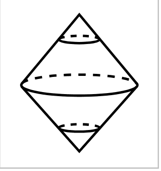
X = Sn , when SX = Sn+1 with the two ‘suspension points’ at the north and south poles of Sn+1 , the points (0, ··· , 0, ±1) (17)

say X=S^1 (circle), then SX = S^2 (sphere)), with north and south pole points as (0,0,-1) and (0,0,+1).

The dimension is raised.

cone CX = (X × I)/(X × {0}) (18)

not only spaces but also maps can be suspended (18)

Join

cone CX is the union of all line segments joining points of X to an external vertex (18)

suspension SX is the union of all line segments joining points of X to two external vertices (18)

given X and a second space Y , one can define the space of all line segments joining points in X to points in Y . This is the join X ∗ Y (18)

an iterated join X1 ∗ ··· ∗ Xn can be constructed as the space of formal linear combinations t1x1 + ··· + tnxn with 0 ≤ ti ≤ 1 and t1 + ··· + tn = 1 (18)

Instead of just 2 spaces X_1 and X_2 (here we called them X and Y), 

say we have n spaces X_1, X_2,...,X_n.

Xi is just a point (18)

Now make each of them as just a point.

join of two points is a line segment (18)

1-simplex.

join of three points is a triangle, (18)

2-simplex.

join of four points is a tetrahedron (18)

3-simplex.

join of n points is a convex polyhedron of dimension n − 1 called a simplex (18)

n points are the n standard basis vectors for Rn , then their join is the (n − 1) dimensional simplex (18)

n-1-simplex.

each Xi is S0 , two points (18)

Rn (18)

Say R^3 then 

(+-1,0,0) (0,+-1,0) (0,0,+-1)

join X1 ∗ ··· ∗ Xn is the union of 2n copies of the simplex ∆n−1 (18)

2^3 = 8 copies of the 2-simplex

radial projection from the origin gives a homeomorphism between X1 ∗ ··· ∗ Xn and Sn−1 (18)

Radial projection means just push each point on the simplex to unit distance from the center.

Therefore,

Join of n number of S^0 spaces is n-1-sphere.

X and Y are CW complexes, then there is a natural CW structure on X ∗ Y having the subspaces X and Y as subcomplexes, with the remaining cells being the product cells of X × Y × (0, 1) (19)

Wedge Sum

spaces X and Y with chosen points x0 ∈ X and y0 ∈ Y , then the wedge sum X ∨ Y is the quotient of the disjoint union X ∐ Y obtained by identifying x0 and y0 to a single point (19)

S1 ∨ S1 is homeomorphic to the figure ‘8’ (19)

Smash Product

smash product X ∧ Y is then defined to be the quotient X × Y /X ∨ Y (19)

Sm ∧Sn has a cell structure with just two cells, of dimensions 0 and m+n , hence Sm ∧Sn = Sm+n (19)

when m = n = 1 we see that collapsing longitude and meridian circles of a torus to a point produces a 2 sphere (19)

Torus is made of 

1 0-cell 2 1-cells 1 2-cell

after collapsing the 2 1-cells to a point, the boundary of the 2-cells gets collapsed to a point and we now have a 2-sphere.

Now,

1 0-cell 1 2-cell

Therefore, S^1 A S^1 has cell structure with just 2 cells of dim 0 and 2.

Two Criteria for Homotopy Equivalence

main tool we used for constructing homotopy equivalences was the fact that a mapping cylinder deformation retracts onto its ‘target’ end (19)

If two spaces deformation retracts to the same space, they are homotopy equivalent.

one can often produce homotopy equivalences between rather different-looking spaces (19)

Like the three graphs example.

first involves collapsing certain subspaces to points (19)

second involves varying the way in which the parts of a space are put together (19)

Collapsing Subspaces

If (X, A) is a CW pair consisting of a CW complex X and a contractible subcomplex A , then the quotient map X→X/A is a homotopy equivalence (20)

The quotient map shows homotopy equivalence.

collapsing the middle edge of the first and third graphs produces the second graph (20)

Instead of deformation retraction idea from the same space, here's a quick way to check,

using the collapsing subspace method.

graph (20)

1-dimensional CW complex.

until all edges of X are loops, and then each component of X is either an isolated vertex or a wedge sum of circles (20)

two such graphs, having only one vertex in each component, can be homotopy equivalent if they are not in fact just isomorphic graphs (20)

Isomorphic means exact same graphs, other than vertex naming.

Before collapsing, two graphs can be homotopy equivalent but not isomorphic. But after collapsing they will be homotopy equivalent and isomorphic.

wedge sum ∨ m S1 of m circles is not homotopy equivalent to ∨ n S1 if m ≠ n (20)

∨ m S1 has Euler characteristic 1−m (20)

Number of even-dim cell is 1 (one point at wedge)

Number of odd-dim cell is m (m 1-spheres aka m circles)

it is a rather nontrivial theorem that the Euler characteristic of a space depends only on its homotopy type (20)

Even though euler characteristic depends on counting the cells in even and odd dimensions of the CW complex, it really does depend on the homotopy only and not on the way we decompose the CW cell.

Although, the proof for showing this is hard.

algebraic invariant that works equally well for graphs, and whose rigorous development requires less effort than the Euler characteristic, is the fundamental group of a space (20)

Instead of assigning a number like euler characteristic, we assign an algebraic object called group.

This is going to help us prove the homotopy of spaces trivially.

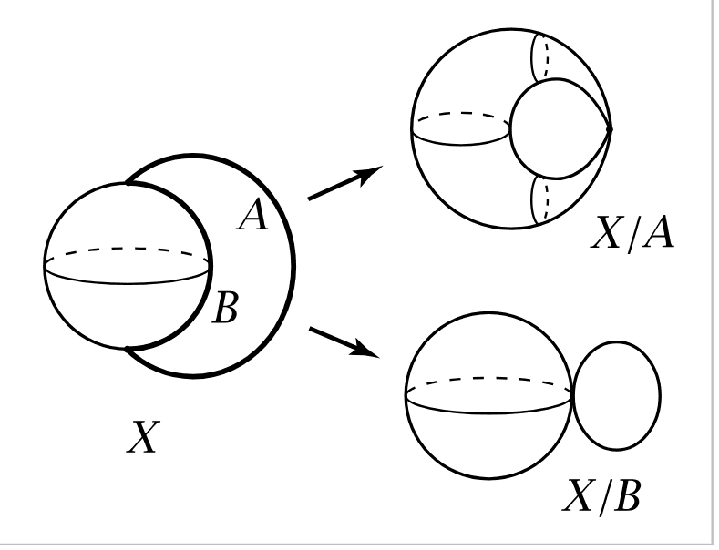
S2 as a 2 cell (20)

This is the only thing that's not contractible.

X/A and X/B are homotopy equivalent to X (21)

A and B are subspaces of X and are contractible. 

So X/A and X/B are homotopy equivalent to X.

S2/S0 and S1 ∨ S2 are homotopy equivalent (21)

intersection points are then the 0 cells, (21)

1 cells are the rest of the longitudinal circle and the boundary circles of the meridional disks (21)

2 cells are the remaining regions of the torus and the interiors of the meridional disks (21)

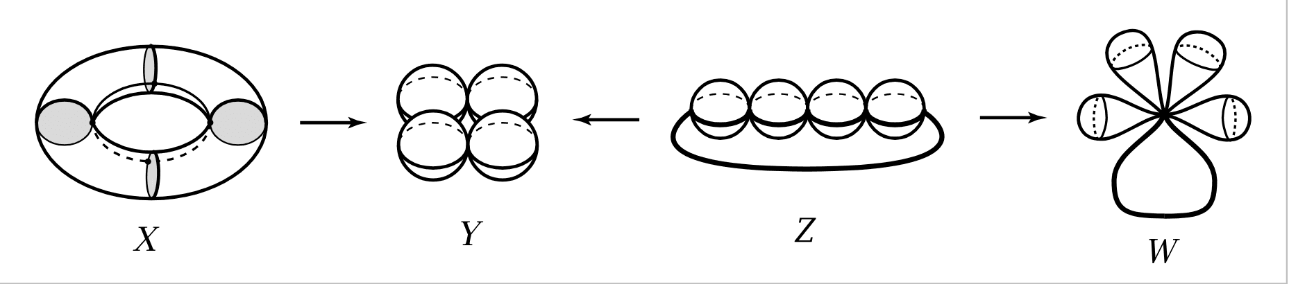
X be a CW complex and x0 ∈ X a 0 cell. Inside the suspension SX we have the line segment {x0}× I , and collapsing this to a point yields a space ΣX homotopy equivalent to SX , called the reduced suspension of X (21)

S1 ∨ S1 (21)

Two bangles joint at a point.

ordinary suspension SX is the union of two spheres intersecting along the arc {x0}× I (21)

2 balls connected by a string.

reduced suspension ΣX is S2 ∨ S2 (21)

2 balls joint at a point.

Σ(X ∨ Y ) = ΣX ∨ ΣY for arbitrary CW complexes X and Y (21)

reduced suspension ΣX is actually the same as the smash product X ∧ S1 (21)

Smashing a space X with a circle, is the same as taking a reduced suspension of X.

Attaching Spaces

start with a space X0 and another space X1 that we wish to attach to X0 by identifying the points in a subspace A ⊂ X1 with points of X0 (22)

Attach points on X_0 with points on subspace A in X_1.

map f : A→X0 , for then we can form a quotient space of X0 ∐ X1 by identifying each point a ∈ A with its image f (a) ∈ X0 (22)

X0 ⊔f X1 , the space X0 with X1 attached along A via f (22)

A is subspace of X_1.

mapping cone Cf = Y ⊔f CX where CX is the cone (X × I)/(X × {0}) and we attach this to Y along X × {1} via the identifications (x, 1) ∼ f (x) (22)

Just like mapping cylinder, but collapse the copy of X to a point.

More like suspension on one side and attach on another.

If (X1, A) is a CW pair and the two attaching maps f , g : A→X0 are homotopic, then X0 ⊔f X1 ≃ X0 ⊔g X1 (22)

attaching map is homotopic to a constant map, and attaching S2 to S1 via a constant map of A yields S1 ∨ S2 (22)

obtained from a circle by attaching n 2 spheres along arcs, so the necklace is homotopy equivalent (22)

slide these attaching points around the circle until they all coincide, producing the wedge sum (22)

X/A ≃ X ∪ CA , the mapping cone of the inclusion A ֓ X (23)

Instead of collapsing a subspace (LHS), we can attaching to a contractible gadget (RHS).

S n /S i ≃S n ∨S i+1 for i < n (23)

Like a S^2 and S^0 will become like sphere and bangle attached at a point

Ultimately, this section summary:

collapsing the S^0 in S^2 Is the same homotopy as attaching the CS^0 in S^2.

The Homotopy Extension Property